install.packages("mice")Exercise 3
Begin this practical by setting the maximum line length in R-Studio to 80 characters.
- Go to Preferences (or Global Options under Tools) –> Code –> Display.
- Tick the Show margin box.
- Set the Margin column to 80.
Data I/O
Install the mice package
Use the install.packages() function to install the the mice package.
If all went well, you will receive a message in the console telling you that the package has been installed.
Load the mice package
Use the library() function to load the mice package.
library(mice)- Installing the package only makes the package available on your machine.
- You have to load the package every time you want to use it in a new R session.
View the mammalsleep data
Most packages have datasets included. Open the mammalsleep dataset from the mice package in two ways:
- By evaluating its name,
mammalsleep, directly - By using the
View()function
# I'm not actually running these lines because the results would clutter
# this document too much.
mammalSleep
View(mammalSleep)
Using View() is preferred for inspecting large datasets because View() opens the dataset in a spreadsheet-like window.
Write the mammalsleep dataset to disk
Save the mammalsleep dataset that you viewed above to your working directory.
- Save the data as a tab-delimited text file.
- Use the
.character as the decimal separator. - Name the file
mammalsleep.txt
write.table(mammalsleep,
            file = "mammalsleep.txt",
            sep = "\t",
            dec = ".",
row.names = FALSE)- The command
sep = "\t"creates a tab-delimited file - The command
dec = "."specifies the.character as the decimal seperator (instead of a comma). - The command
row.names = FALSEtells R not to include row names in the exported file.
Read the mammalsleep.txt file from disk
Read in the data that you just saved to disk and save it as a new R object called sleepdata.
sleepdata <- read.table("mammalsleep.txt",
                        sep = "\t",
                        dec = ".",
                        header = TRUE,
stringsAsFactors = TRUE)- The command
sep = "\t"indicates that the file is tab-delimited - The command
dec = "."indicates that a.is used as the decimal seperator - The command
header = TRUEtells R that the first row of data contains the variable names - The
stringsAsFactors = TRUEcommand will automatically convert any character variables to factors
You can read files that live in the working directory by specifying only the file name (with the file extension). To read files that live in any other location, you need to specify the full file path (either relative to the working directory or an absolute path). To find the current working directory, you can run getwd(). To change the working directory, you can use setwd(). One benefit of using RStudio projects is that the working directory is automatically set to the main project directory.
There are many packages that facilitate data I/O from other statistical software packages such as:
- SPSS (e.g.
read_spss()from the haven package) - Mplus (routines in the MplusAutomation package)
- Stata (
read.dta()in the foreign package) - SAS (
sasxport.get()from the Hmisc package)
There are also packages to read data from spreadsheet software such as MS Excel (read.xlsx() from the xlsx package).
For a short guide on importing multiple file formats into R, see this page.
Working with Data
Explore the data
The dataset you’ve just imported contains the sleep data from Allison and Cicchetti (1976).
- Explore these data, and familiarize yourself with the characteristics of the dataset.
There is no completely right or wrong way to go about exploring a dataset, but the following commands represent some potential options.
# Call up the documentation for the original dataset in the mice package:
?mammalsleep
# Show the data structure:
str(sleepdata)'data.frame': 62 obs. of 11 variables:
$ species: Factor w/ 62 levels "African elephant",..: 1 2 3 4 5 6 7 8 9 10 ...
$ bw : num 6654 1 3.38 0.92 2547 ...
$ brw : num 5712 6.6 44.5 5.7 4603 ...
$ sws : num NA 6.3 NA NA 2.1 9.1 15.8 5.2 10.9 8.3 ...
$ ps : num NA 2 NA NA 1.8 0.7 3.9 1 3.6 1.4 ...
$ ts : num 3.3 8.3 12.5 16.5 3.9 9.8 19.7 6.2 14.5 9.7 ...
$ mls : num 38.6 4.5 14 NA 69 27 19 30.4 28 50 ...
$ gt : num 645 42 60 25 624 180 35 392 63 230 ...
$ pi : int 3 3 1 5 3 4 1 4 1 1 ...
$ sei : int 5 1 1 2 5 4 1 5 2 1 ...
$ odi : int 3 3 1 3 4 4 1 4 1 1 ...# Show summaries of the univariate distributions:
summary(sleepdata) species bw brw
African elephant : 1 Min. : 0.005 Min. : 0.14
African giant pouched rat: 1 1st Qu.: 0.600 1st Qu.: 4.25
Arctic Fox : 1 Median : 3.342 Median : 17.25
Arctic ground squirrel : 1 Mean : 198.790 Mean : 283.13
Asian elephant : 1 3rd Qu.: 48.203 3rd Qu.: 166.00
Baboon : 1 Max. :6654.000 Max. :5712.00
(Other) :56
sws ps ts mls
Min. : 2.100 Min. :0.000 Min. : 2.60 Min. : 2.000
1st Qu.: 6.250 1st Qu.:0.900 1st Qu.: 8.05 1st Qu.: 6.625
Median : 8.350 Median :1.800 Median :10.45 Median : 15.100
Mean : 8.673 Mean :1.972 Mean :10.53 Mean : 19.878
3rd Qu.:11.000 3rd Qu.:2.550 3rd Qu.:13.20 3rd Qu.: 27.750
Max. :17.900 Max. :6.600 Max. :19.90 Max. :100.000
NA's :14 NA's :12 NA's :4 NA's :4
gt pi sei odi
Min. : 12.00 Min. :1.000 Min. :1.000 Min. :1.000
1st Qu.: 35.75 1st Qu.:2.000 1st Qu.:1.000 1st Qu.:1.000
Median : 79.00 Median :3.000 Median :2.000 Median :2.000
Mean :142.35 Mean :2.871 Mean :2.419 Mean :2.613
3rd Qu.:207.50 3rd Qu.:4.000 3rd Qu.:4.000 3rd Qu.:4.000
Max. :645.00 Max. :5.000 Max. :5.000 Max. :5.000
NA's :4 # Show (rounded) bivariate correlations (excluding the ID column):
round(cor(sleepdata[, -1], use = "pairwise.complete.obs"), 2) bw brw sws ps ts mls gt pi sei odi
bw 1.00 0.93 -0.38 -0.11 -0.31 0.30 0.65 0.06 0.34 0.13
brw 0.93 1.00 -0.37 -0.11 -0.36 0.51 0.75 0.03 0.37 0.15
sws -0.38 -0.37 1.00 0.51 0.96 -0.38 -0.59 -0.32 -0.54 -0.48
ps -0.11 -0.11 0.51 1.00 0.73 -0.30 -0.45 -0.45 -0.54 -0.58
ts -0.31 -0.36 0.96 0.73 1.00 -0.41 -0.63 -0.40 -0.64 -0.59
mls 0.30 0.51 -0.38 -0.30 -0.41 1.00 0.61 -0.10 0.36 0.06
gt 0.65 0.75 -0.59 -0.45 -0.63 0.61 1.00 0.20 0.64 0.38
pi 0.06 0.03 -0.32 -0.45 -0.40 -0.10 0.20 1.00 0.62 0.92
sei 0.34 0.37 -0.54 -0.54 -0.64 0.36 0.64 0.62 1.00 0.79
odi 0.13 0.15 -0.48 -0.58 -0.59 0.06 0.38 0.92 0.79 1.00# Show the first six rows:
head(sleepdata) species bw brw sws ps ts mls gt pi sei odi
1 African elephant 6654.000 5712.0 NA NA 3.3 38.6 645 3 5 3
2 African giant pouched rat 1.000 6.6 6.3 2.0 8.3 4.5 42 3 1 3
3 Arctic Fox 3.385 44.5 NA NA 12.5 14.0 60 1 1 1
4 Arctic ground squirrel 0.920 5.7 NA NA 16.5 NA 25 5 2 3
5 Asian elephant 2547.000 4603.0 2.1 1.8 3.9 69.0 624 3 5 4
6 Baboon 10.550 179.5 9.1 0.7 9.8 27.0 180 4 4 4# Show the last six rows:
tail(sleepdata) species bw brw sws ps ts mls gt pi sei odi
57 Tenrec 0.900 2.6 11.0 2.3 13.3 4.5 60 2 1 2
58 Tree hyrax 2.000 12.3 4.9 0.5 5.4 7.5 200 3 1 3
59 Tree shrew 0.104 2.5 13.2 2.6 15.8 2.3 46 3 2 2
60 Vervet 4.190 58.0 9.7 0.6 10.3 24.0 210 4 3 4
61 Water opossum 3.500 3.9 12.8 6.6 19.4 3.0 14 2 1 1
62 Yellow-bellied marmot 4.050 17.0 NA NA NA 13.0 38 3 1 1Since mammalsleep is an R dataset, it should have a help file. The documentation for the mammalsleep dataset may yield valuable insight about the origin of the data and the variables included therein.
The functions head() and tail() are very useful. If something went from with reading the data, you can often tell very quickly by looking at the first or last rows (do they look like you expected)?
The str function is a good way to get a quick overview of the measurement levels in a dataset.
- Notice how the information returned by the
str()function looks very similar to the information you see in RStudio’s Environment tab. - The Environment tab is simply reporting the results of the
str()function in a pretty format.
Notice that sleepdata is a data frame. The read.table() function will return the data it reads as a data frame.
One thing that may have caught your attention is the relation between ts, ps and sws. This relation is deterministic: total sleep (ts) is the sum of paradoxical sleep (ps) and short-wave sleep (sws). If you were to model these data, you would need to account for such relations in your analysis.
Subset the data
Some animals were not used by Allison and Cicchetti (1976).
- Exclude the following animals from
sleepdata:- Echidna
- Lesser short-tailed shrew
- Musk shrew
- Save the dataset as
sleepdata2
There are at least three ways to exclude these animals from the dataset.
The first two approaches both require us to use the species variable to create a logical vector flagging the rows to drop.
exclusions <- sleepdata$species %in%
c("Echidna", "Lesser short-tailed shrew", "Musk shrew")- The first approach uses standard, base R subsetting procedures:
# Negate the logical vector to select all rows other than the exclusions:
sleepdata2 <- sleepdata[!exclusions, ]- The second approach uses the
filter()function from thedplyrpackage:
library(dplyr)
sleepdata2 <- filter(sleepdata, !exclusions)- The third approach uses the row numbers directly
- You will need to manually figure out which row numbers you want to exclude
sleepdata2 <- sleepdata[-c(16, 32, 38), ]Note that the row number option requires less code, but the first two options have much lower probabilities for error.
- If the dataset changes or the rows are sorted differently, the row number option may not work correctly (i.e., you’d exclude the wrong cases).
- Since you find the rows programatically in the first two options, they are much more robust to changes in the data.
Plot brain weight as a function of species
Use the sleepdata2 dataset and base R graphics routines to create a plot of brain weight against species.
plot(brw ~ species, data = sleepdata2)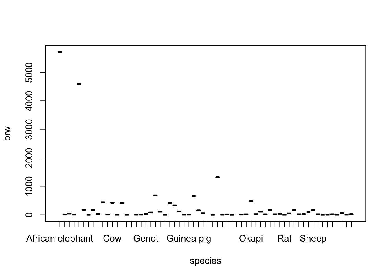
Conditional case selection
Some animals have much heavier brains than other animals. Find the names of all animals that have a brain weight larger than 1 standard deviation above the mean brain weight.
# Create a logical vector flagging the rows with extreme brain weights:
bigBrains <- sleepdata2$brw > (mean(sleepdata2$brw) + sd(sleepdata2$brw))

# Extract the names from any row flagged by the above vector:
as.character(sleepdata2$species[bigBrains])
[1] "African elephant" "Asian elephant" "Man" Plot of big-brained animals
Replicate the plot from @cref-plot with only the animals you flagged in @cref-flag
- Do not plot any information about the other animals.
A naive attempt may simply try to run the same plotting code with a subset of the data.
plot(brw ~ species, data = sleepdata2[bigBrains, ])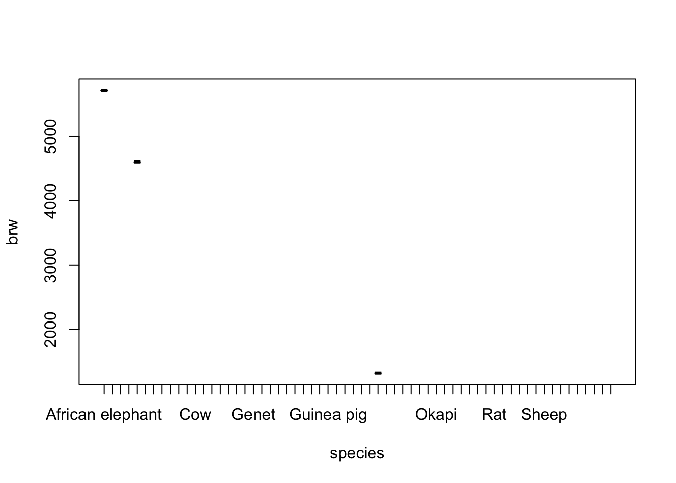
The downside to this approach is that it still includes all animals on the x-axis. The original factor labels for species remain unchanged in the subset of the original data.
levels(sleepdata2$species[bigBrains]) [1] "African elephant" "African giant pouched rat"
[3] "Arctic Fox" "Arctic ground squirrel"
[5] "Asian elephant" "Baboon"
[7] "Big brown bat" "Brazilian tapir"
[9] "Cat" "Chimpanzee"
[11] "Chinchilla" "Cow"
[13] "Desert hedgehog" "Donkey"
[15] "Eastern American mole" "Echidna"
[17] "European hedgehog" "Galago"
[19] "Genet" "Giant armadillo"
[21] "Giraffe" "Goat"
[23] "Golden hamster" "Gorilla"
[25] "Gray seal" "Gray wolf"
[27] "Ground squirrel" "Guinea pig"
[29] "Horse" "Jaguar"
[31] "Kangaroo" "Lesser short-tailed shrew"
[33] "Little brown bat" "Man"
[35] "Mole rat" "Mountain beaver"
[37] "Mouse" "Musk shrew"
[39] "N. American opossum" "Nine-banded armadillo"
[41] "Okapi" "Owl monkey"
[43] "Patas monkey" "Phanlanger"
[45] "Pig" "Rabbit"
[47] "Raccoon" "Rat"
[49] "Red fox" "Rhesus monkey"
[51] "Rock hyrax (Hetero. b)" "Rock hyrax (Procavia hab)"
[53] "Roe deer" "Sheep"
[55] "Slow loris" "Star nosed mole"
[57] "Tenrec" "Tree hyrax"
[59] "Tree shrew" "Vervet"
[61] "Water opossum" "Yellow-bellied marmot" The plot() function uses all 62 factor levels to generate the x-axis even though 59 levels are empty.
To get rid of the unused factor levels, we can use the factor() function.
sleepdata3 <- sleepdata2[bigBrains, ]
sleepdata3$species <- factor(sleepdata3$species)
levels(sleepdata3$species)
[1] "African elephant" "Asian elephant" "Man" Now we can create the plot that we wanted:
plot(brw ~ species, data = sleepdata3)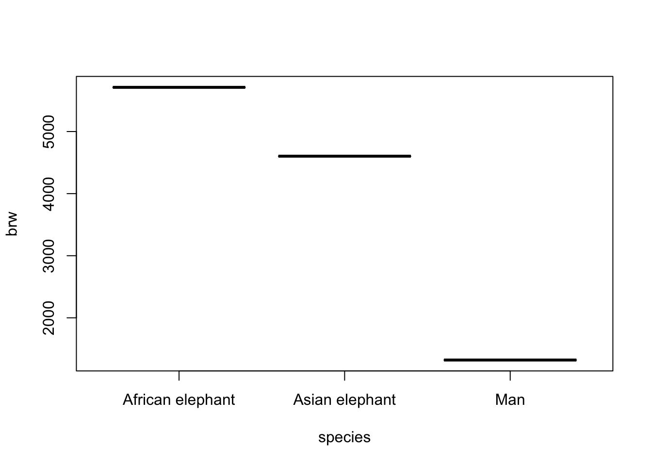
Workspace I/O
Save the current workspace
Now that we have imported some data and done some analyses and data manipulations, we may want to save the current workspace (i.e. the current state of our R session). Saving the workspace will save everything in the R session exactly as it exists at the moment of saving. So, we can easily continue from this exact state at a later time. All we need to do is re-load the saved workspace file.
Use the save.image() function to save the entirety of the current workspace.
- Name the workspace image
practical3.RData.
Also, use the save() function to save the sleepdata dataset as a separate workspace.
- Name this workspace
sleepdata.RData.
save.image("practical3.RData")
save(sleepdata, file = "sleepdata.RData")
Clear the workspace
Run the following command to clear the workspace.
rm(list = ls(all = TRUE))This is a very handy line of code to memorize. It will clear nearly everything from your current workspace. If you’re curious about how it does so, check the help files for the rm() and ls() functions.
Load a saved workspace
Use the load() function to load the practical3.RData workspace that you saved in @cref-save.
load("practical3.RData")Load a saved dataset
- Use the
rm()function to remove thesleepdatadataset from the environment. - Use the
load()function to reload thesleepdatadataset from the sleepdata.RData workspace you saved in @cref-save
rm(sleepdata)
load("sleepdata.RData")
A better way to read/write R data objects
You may have noticed that when you load a dataset with read.table(), you assign the result to a new R object. However, when you load a dataset saved as a workspace using the load() function, you cannot rename the resulting R object.
When saving an R object with the save() function and loading it with the load() function, the object keeps the name it had when saved. When saving and loading individual data objects, this behavior is rarely desirable.
The saveRDS() and readRDS() functions allow us to save and load R objects in R Data Set (RDS) format.
- Objects stored in RDS format do not keep their original names.
- We have to give the saved object to a new name when we load it with the
readRDS()function. - This workflow is more transparent than the behavior of
save()andload()and better follows the R philosophy of assigning values to objects.
If you need to save individual R objects (i.e., not an entire workspace image), you should probably save them as RDS files and not RData workspaces.
- Use the
saveRDS()function to save thesleepdataobject as sleepdata.rds. - Use the
readRDS()function to load the sleepdata.rds file and assign it to thesleepdata4object.
saveRDS(sleepdata, "sleepdata.rds")
sleepdat4 <- readRDS("sleepdata.rds")
A Useful Package for Data I/O
If R is not (yet) your preferred data-analysis software, you are probably accustomed to processing your data in some other software and storing data in formats other than RData or RDS. In R, there are many facilities for importing and exporting data with diverse formats.
Here, I want to specifically highlight the haven package written by Hadley Wickham. The haven package provides many useful functions to import and export data from software such as Stata, SAS, and SPSS.
End of Exercise 3
—
Copyright Hanne Oberman, 2025 - CC BY-NC-SA 4.0
Materials developed by Amices team - Methodology & Statistics - Utrecht University