Imputation of Incomplete Multilevel Data with R

Hanne Oberman

PhD candidate at Utrecht University

Incomplete multilevel data

\[ \text{multilevel structure } \times \text{ missing data } \]

Missingness

Missing data methods

• Prevention
• Ad-hoc methods, e.g., single imputation, list-wise deletion
• Weighting methods
• Likelihood methods, EM-algorithm
• Multiple imputation

Multiple imputation

• Works with item non-response
• Does not assume MCAR
• Does not over-complicate the analysis model

Ingredients

• Incomplete data
• Assumed missingness mechanism
• Known analysis model

Case study (Hox et al., 2018)

\[\begin{align} \text{popularity}_{ij} = &\gamma_{00}+ \gamma_{10} \text{gender}_{ij} + \gamma_{20} \text{extraversion}_{ij} + \\ &\gamma_{01} \text{experience}_j + \gamma_{21} \text{extraversion}_{ij} \times \text{experience}_j + \\ &u_{2j} \text{extraversion}_{ij} + u_{0j}+ e_{ij} \end{align}\]

Setup

set.seed(123)         # for reproducibility
library(mice)         # for imputation
library(miceadds)     # for imputation
library(ggmice)       # for visualization
library(ggplot2)      # for visualization
library(dplyr)        # for data wrangling
library(lme4)         # for multilevel modeling
library(broom)        # for tidying model output
library(broom.mixed)  # for tidying model output
str(dat)

'data.frame':   2000 obs. of  7 variables:
 $ unit_id        : num  1 2 3 4 5 6 7 8 9 10 ...
 $ cluster_id     : num  1 1 1 1 1 1 1 1 1 1 ...
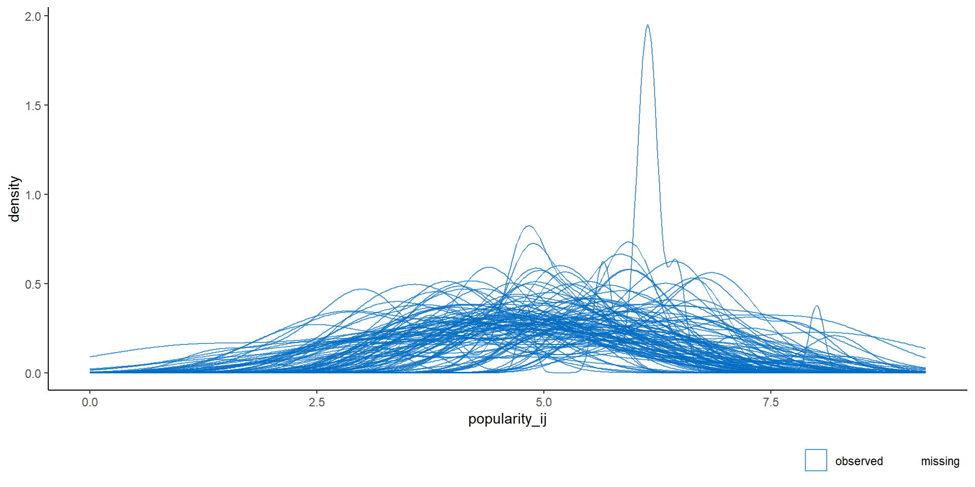
 $ popularity_ij  : num  6.3 4.9 5.3 4.7 6 4.7 5.9 NA 5.2 NA ...
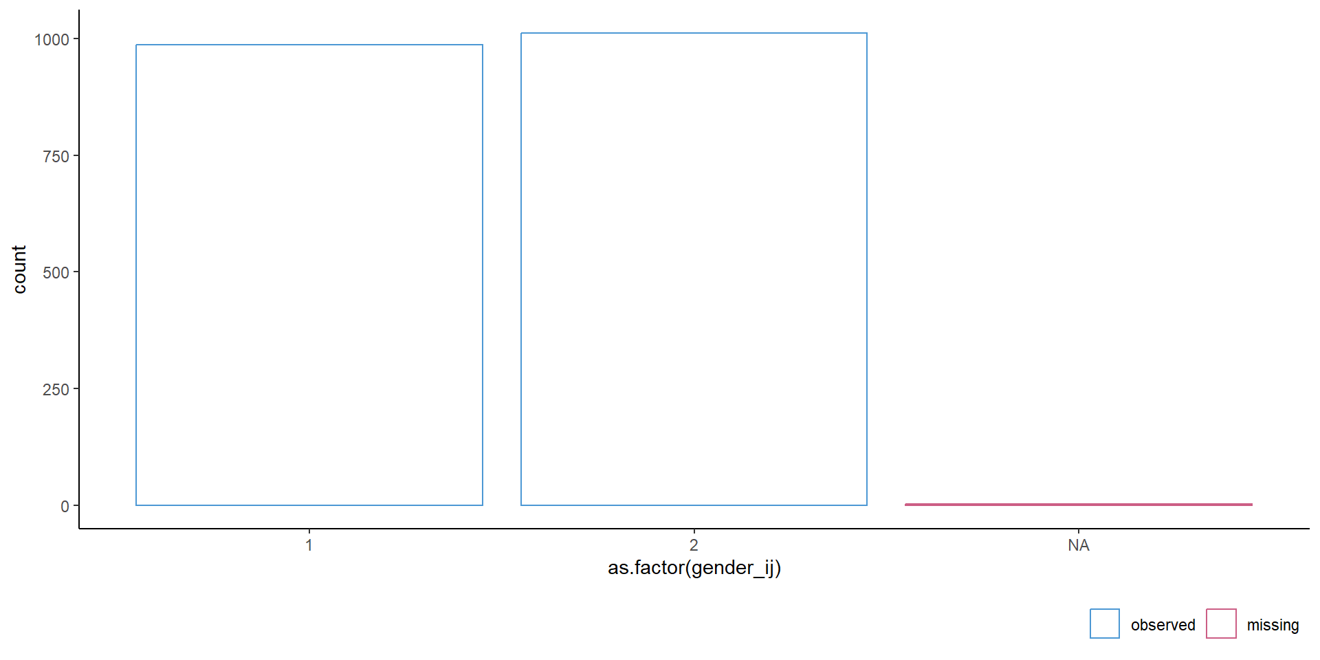
 $ gender_ij      : num  2 1 2 2 2 1 1 1 1 1 ...
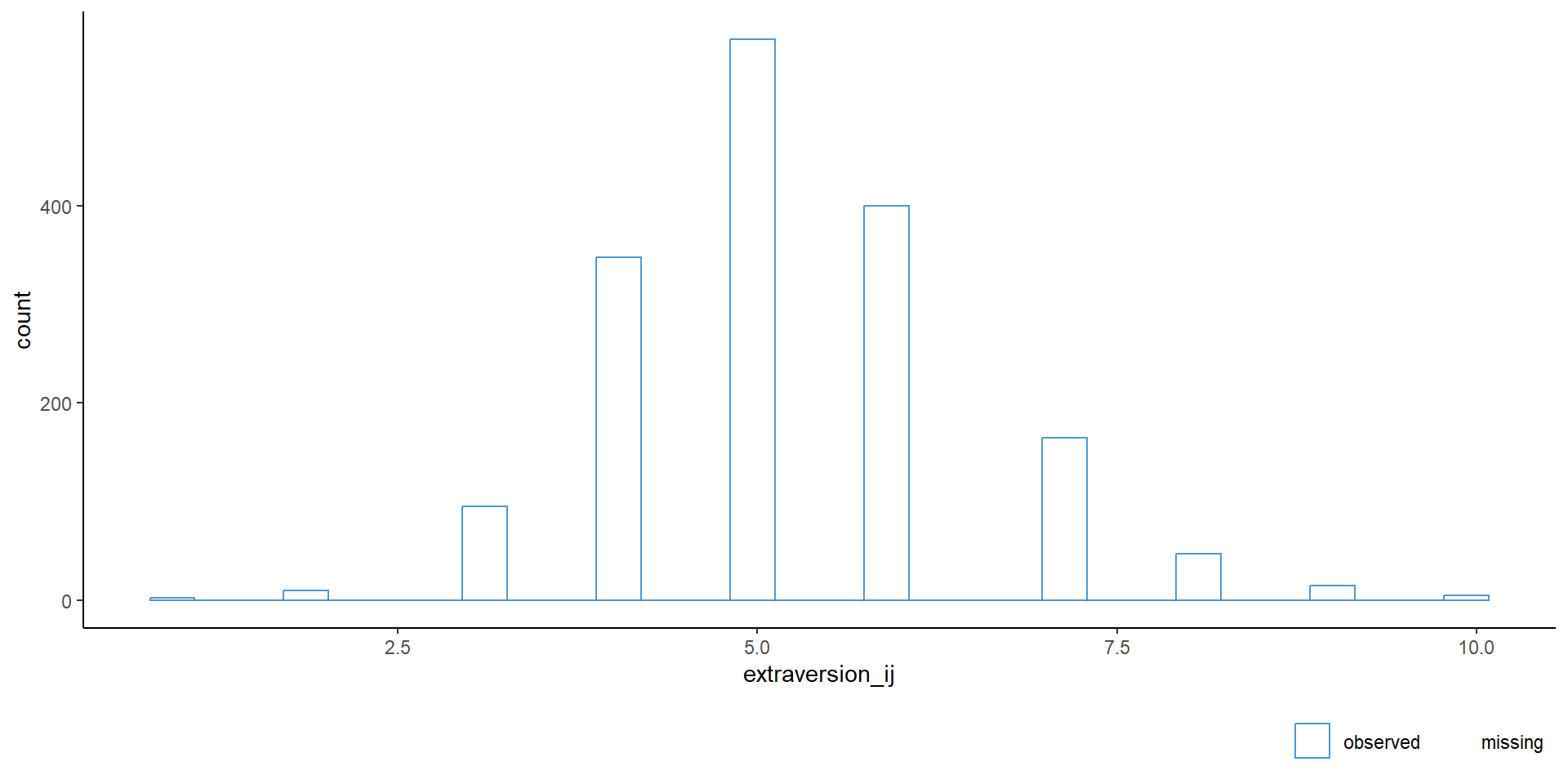
 $ extraversion_ij: num  5 7 4 3 5 4 5 NA 5 5 ...
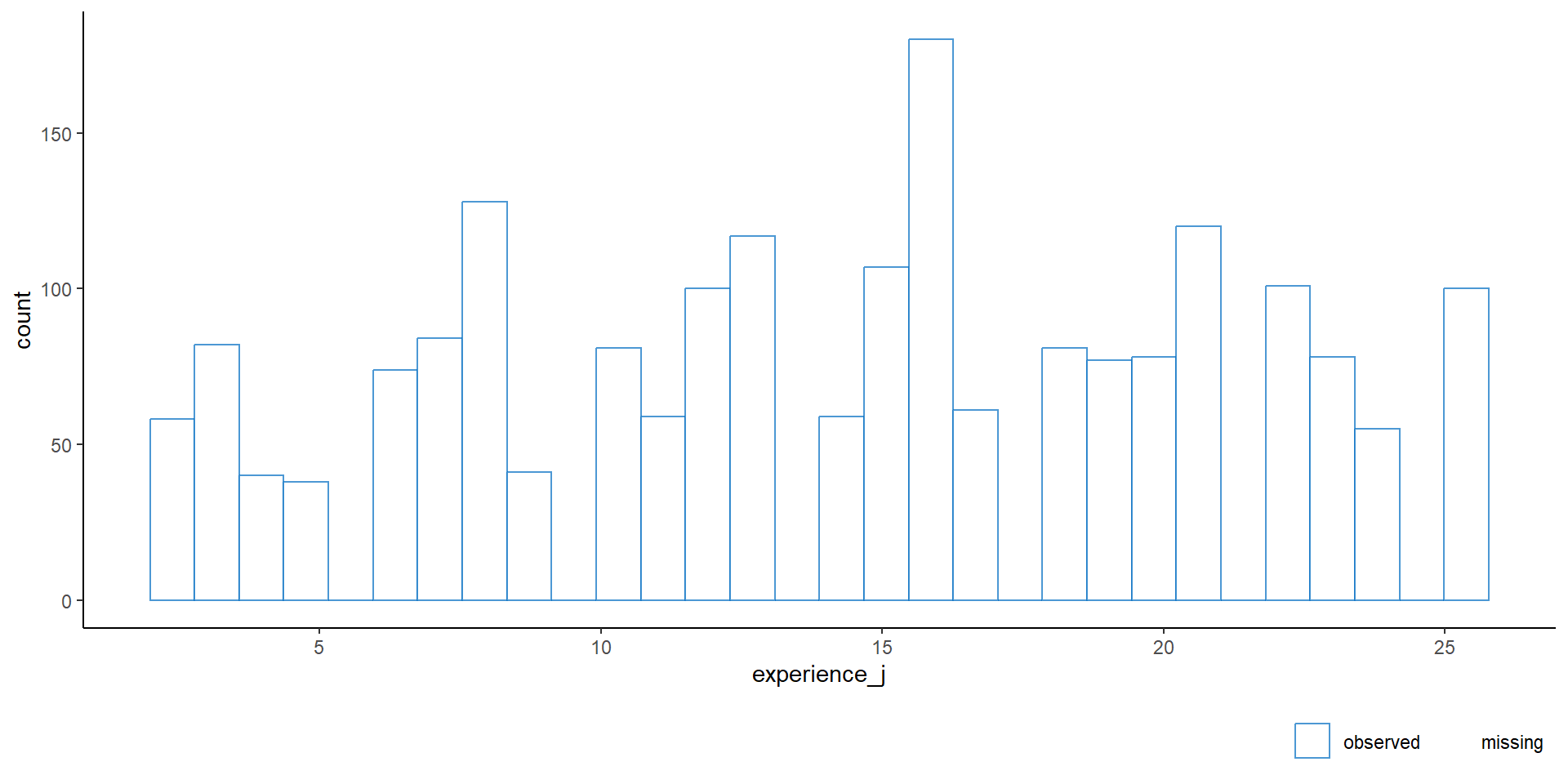
 $ experience_j   : num  24 NA 24 24 24 24 24 24 24 24 ...
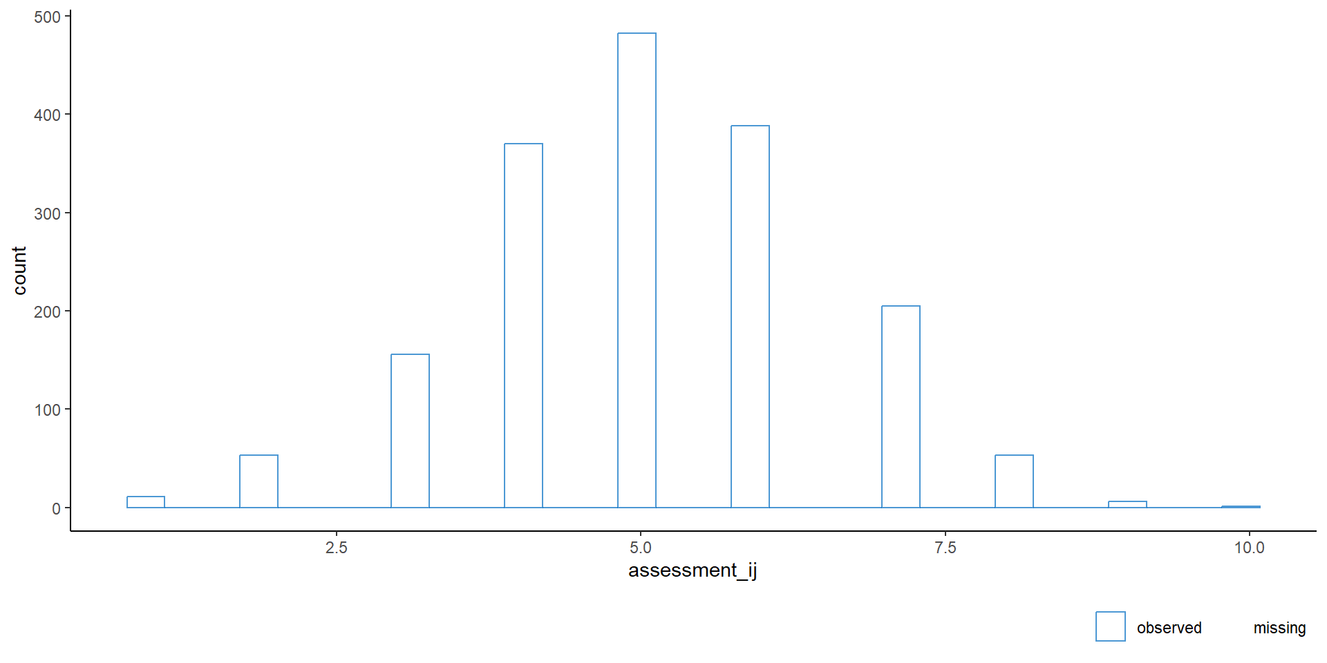
 $ assessment_ij  : num  6 NA 6 5 6 5 5 NA 5 3 ...

Missing data pattern

plot_pattern(dat, square = FALSE)

Imputation model building

plot_corr(dat, square = FALSE)

Default imputation methods

meth <- make.method(dat)
meth

        unit_id      cluster_id   popularity_ij       gender_ij extraversion_ij 
             ""              ""           "pmm"           "pmm"           "pmm" 
   experience_j   assessment_ij 
          "pmm"           "pmm" 

Outcome variable: popularity

ggmice(dat, aes(popularity_ij, group = cluster_id)) + 
  geom_density()

meth["popularity_ij"] <- "2l.norm"

Unit-level variable: gender

ggmice(dat, aes(as.factor(gender_ij))) + 
  geom_bar(position = "stack", fill = "white")

meth["gender_ij"] <- "2l.bin"

Unit-level variable: extraversion

ggmice(dat, aes(extraversion_ij)) + 
  geom_histogram(fill = "white")

meth["extraversion_ij"] <- "2l.pmm"

Auxiliary variable: teacher assessment

ggmice(dat, aes(assessment_ij)) + 
  geom_histogram(fill = "white")

meth["assessment_ij"] <- "2l.pmm"

Cluster-level variable: teacher experience

ggmice(dat, aes(experience_j)) + 
  geom_histogram(fill = "white")

meth["experience_j"] <- "2lonly.pmm"

Cross-level interaction: pupil extraversion \(\times\) teacher experience

dat$interaction <- NA
meth["interaction"] <- "~ I(extraversion_ij * experience_j)"
meth

                              unit_id                            cluster_id 
                                   ""                                    "" 
                        popularity_ij                             gender_ij 
                            "2l.norm"                              "2l.bin" 
                      extraversion_ij                          experience_j 
                             "2l.pmm"                          "2lonly.pmm" 
                        assessment_ij                           interaction 
                             "2l.pmm" "~ I(extraversion_ij * experience_j)" 

Default predictor matrix

pred <- quickpred(dat)
plot_pred(pred, method = meth, square = FALSE)

Outcome variable: popularity

# clustering variable
pred["popularity_ij", "cluster_id"] <- -2
# fixed effect for gender, random effect for extraversion
pred["popularity_ij", "gender_ij"] <- 1
pred["popularity_ij", "extraversion_ij"] <- 2
# add disaggregated cluster means
pred["popularity_ij", "gender_ij"] <- 3
pred["popularity_ij", "extraversion_ij"] <- 4
# cluster-level variable
pred["popularity_ij", "experience_j"] <- 1
# interaction term
pred["popularity_ij", "interaction"] <- 1
# auxiliary variable
pred["popularity_ij", "assessment_ij"] <- 1

Predictor variables

# clustering variable
pred[, "cluster_id"] <- -2
# outcome variable
pred[, "popularity_ij"] <- 1
# clean up predictor matrix
pred[, "interaction"] <- 0
pred[, "unit_id"] <- 0
diag(pred) <- 0

Predictor matrix

plot_pred(pred, method = meth, square = FALSE)

Impute the data

imp <- mice(
  dat, 
  m = 1, 
  method = meth, 
  predictorMatrix = pred,
  maxit = 1)

Error

iter imp variable
  1   1  popularity_ij  gender_ij  extraversion_ij  experience_jError in .imputation.level2(y = y, ry = ry, x = x, type = type, wy = wy,  : 
  Method 2lonly.pmm found the following clusters with partially missing
  level-2 data: 1
  Method 2lonly.mean can fix such inconsistencies.
In addition: Warning message:
In mice.impute.2l.bin(y = c(2, 1, 2, 2, 2, 1, 1, 1, 1, 1, 2, 2,  :
  glmer does not run. Simplify imputation model

Edit the methods and re-impute

meth["experience_j"] <- "2lonly.mean"
meth["gender_ij"] <- "2l.pmm"
# re-impute
imp <- mice(
  dat, 
  method = meth, 
  predictorMatrix = pred,
  maxit = 1,
  printFlag = FALSE)

Succes!

Add iterations and evaluate

imp <- mice.mids(imp, maxit = 9, printFlag = FALSE)
plot_trace(imp)

Non-convergence?

plot_pattern(dat, square = FALSE)

Evaluate imputations

• Distribution of imputed values
• Plausibility of imputed values
• Variability between imputations

Outcome variable: popularity (1)

ggmice(imp, aes(.imp, popularity_ij)) + 
  geom_jitter(height = 0)

range(mice::complete(imp)$popularity_ij)

[1]  0.00000 10.19287

Outcome variable: popularity (2)

ggmice(imp, aes(popularity_ij, group = .imp)) + 
  geom_density()

Multivariate visualization

Analyze imputed data

• Complete case analysis
• Sequential model building

Single-level model

cca <- lm(
  popularity_ij ~ 1, 
  data = dat
  )
tidy(cca)

# A tibble: 1 × 5
  term        estimate std.error statistic p.value
  <chr>          <dbl>     <dbl>     <dbl>   <dbl>
1 (Intercept)     5.03    0.0396      127.       0

fit <- with(
  imp,
  lm(popularity_ij ~ 1, data = dat)
  ) |> 
  pool()
tidy(fit)

         term estimate  std.error statistic p.value b       df dfcom
1 (Intercept) 5.033555 0.03963228  127.0065       0 0 1197.882  1200
          fmi lambda m riv        ubar
1 0.001665443      0 5   0 0.001570717

Intercept-only model (1)

fit <- with(
  imp,
  lmer(
    popularity_ij ~ (1 | cluster_id), 
    data = dat, 
    REML = FALSE)
  ) 
pool(fit) |> tidy()

         term estimate std.error statistic p.value b       df dfcom         fmi
1 (Intercept) 5.021201 0.0890947  56.35802       0 0 1195.882  1198 0.001668221
  lambda m riv        ubar
1      0 5   0 0.007937865

Intercept-only model (2)

mitml::testEstimates(as.mitml.result(fit), extra.pars = TRUE)

Call:

mitml::testEstimates(model = as.mitml.result(fit), extra.pars = TRUE)

Final parameter estimates and inferences obtained from 5 imputed data sets.

             Estimate Std.Error   t.value        df   P(>|t|)       RIV       FMI 
(Intercept)     5.021     0.089    56.358       Inf     0.000     0.000     0.000 

                                Estimate 
Intercept~~Intercept|cluster_id    0.690 
Residual~~Residual                 1.193 
ICC|cluster_id                     0.367 

Unadjusted hypothesis test as appropriate in larger samples.

Model with explanatory variables

fit <- with(
  imp,
  lmer(
    popularity_ij ~ gender_ij + extraversion_ij + experience_j + (1 | cluster_id),
    data = dat, 
    REML = FALSE)
  ) 
pool(fit) |> tidy()

             term    estimate   std.error statistic       p.value b       df
1     (Intercept) -0.45459695 0.199053149 -2.283797  2.255904e-02 0 1189.882
2       gender_ij  1.28611143 0.048112155 26.731528 1.120524e-123 0 1189.882
3 extraversion_ij  0.44652838 0.021546495 20.723945  1.056952e-81 0 1189.882
4    experience_j  0.08767041 0.008744419 10.025871  9.120374e-23 0 1189.882
  dfcom         fmi lambda m riv         ubar
1  1192 0.001676611      0 5   0 3.962216e-02
2  1192 0.001676611      0 5   0 2.314779e-03
3  1192 0.001676611      0 5   0 4.642515e-04
4  1192 0.001676611      0 5   0 7.646486e-05

Model with explanatory variables (2)

mitml::testEstimates(as.mitml.result(fit), extra.pars = TRUE)

Call:

mitml::testEstimates(model = as.mitml.result(fit), extra.pars = TRUE)

Final parameter estimates and inferences obtained from 5 imputed data sets.

                 Estimate Std.Error   t.value        df   P(>|t|)       RIV       FMI 
(Intercept)        -0.455     0.199    -2.284       Inf     0.022     0.000     0.000 
gender_ij           1.286     0.048    26.732       Inf     0.000     0.000     0.000 
extraversion_ij     0.447     0.022    20.724       Inf     0.000     0.000     0.000 
experience_j        0.088     0.009    10.026       Inf     0.000     0.000     0.000 

                                Estimate 
Intercept~~Intercept|cluster_id    0.269 
Residual~~Residual                 0.583 
ICC|cluster_id                     0.316 

Unadjusted hypothesis test as appropriate in larger samples.

Model with explanatory variables, extraversion slope random

fit <- with(
  imp,
  lmer(
    popularity_ij ~ gender_ij + extraversion_ij + experience_j + 
      (1  + extraversion_ij | cluster_id), 
    data = dat, 
    REML = FALSE)
  ) 
pool(fit) |> tidy()

             term    estimate   std.error statistic       p.value b       df
1     (Intercept) -0.43804176 0.222237366 -1.971054  4.894959e-02 0 1187.883
2       gender_ij  1.28026787 0.047605007 26.893555 8.201898e-125 0 1187.883
3 extraversion_ij  0.43968176 0.028356053 15.505746  1.603530e-49 0 1187.883
4    experience_j  0.08706721 0.008630314 10.088533  5.090619e-23 0 1187.883
  dfcom         fmi lambda m riv         ubar
1  1190 0.001679427      0 5   0 4.938945e-02
2  1190 0.001679427      0 5   0 2.266237e-03
3  1190 0.001679427      0 5   0 8.040658e-04
4  1190 0.001679427      0 5   0 7.448233e-05

Model with explanatory variables, extraversion slope random (2)

mitml::testEstimates(as.mitml.result(fit), extra.pars = TRUE)

Call:

mitml::testEstimates(model = as.mitml.result(fit), extra.pars = TRUE)

Final parameter estimates and inferences obtained from 5 imputed data sets.

                 Estimate Std.Error   t.value        df   P(>|t|)       RIV       FMI 
(Intercept)        -0.438     0.222    -1.971       Inf     0.049     0.000     0.000 
gender_ij           1.280     0.048    26.894       Inf     0.000     0.000     0.000 
extraversion_ij     0.440     0.028    15.506       Inf     0.000     0.000     0.000 
experience_j        0.087     0.009    10.089       Inf     0.000     0.000     0.000 

                                            Estimate 
Intercept~~Intercept|cluster_id                1.283 
extraversion_ij~~extraversion_ij|cluster_id    0.032 
Intercept~~extraversion_ij|cluster_id         -0.183 
Residual~~Residual                             0.548 
ICC|cluster_id                                 0.701 

Unadjusted hypothesis test as appropriate in larger samples.

Model with with cross-level interaction

fit <- with(
  imp,
  lmer(
    popularity_ij ~ gender_ij + extraversion_ij + experience_j + 
      extraversion_ij:experience_j + (1  + extraversion_ij | cluster_id),  
    data = dat, 
    REML = FALSE)
  ) 
pool(fit) |> tidy()

                          term    estimate   std.error statistic       p.value
1                  (Intercept) -2.33429638 0.311701929 -7.488874  1.351136e-13
2                    gender_ij  1.26491027 0.046825663 27.013184 1.162079e-125
3              extraversion_ij  0.77879482 0.046234259 16.844540  2.986533e-57
4                 experience_j  0.21927052 0.018952063 11.569744  2.074365e-29
5 extraversion_ij:experience_j -0.02386015 0.002955871 -8.072122  1.681341e-15
  b       df dfcom         fmi lambda m riv         ubar
1 0 1186.883  1189 0.001680838      0 5   0 9.715809e-02
2 0 1186.883  1189 0.001680838      0 5   0 2.192643e-03
3 0 1186.883  1189 0.001680838      0 5   0 2.137607e-03
4 0 1186.883  1189 0.001680838      0 5   0 3.591807e-04
5 0 1186.883  1189 0.001680838      0 5   0 8.737174e-06

Model with with cross-level interaction (2)

mitml::testEstimates(as.mitml.result(fit), extra.pars = TRUE)

Call:

mitml::testEstimates(model = as.mitml.result(fit), extra.pars = TRUE)

Final parameter estimates and inferences obtained from 5 imputed data sets.

                              Estimate Std.Error   t.value        df   P(>|t|)       RIV       FMI 
(Intercept)                     -2.334     0.312    -7.489       Inf     0.000     0.000     0.000 
gender_ij                        1.265     0.047    27.013       Inf     0.000     0.000     0.000 
extraversion_ij                  0.779     0.046    16.845       Inf     0.000     0.000     0.000 
experience_j                     0.219     0.019    11.570       Inf     0.000     0.000     0.000 
extraversion_ij:experience_j    -0.024     0.003    -8.072       Inf     0.000     0.000     0.000 

                                            Estimate 
Intercept~~Intercept|cluster_id                0.360 
extraversion_ij~~extraversion_ij|cluster_id    0.001 
Intercept~~extraversion_ij|cluster_id         -0.011 
Residual~~Residual                             0.550 
ICC|cluster_id                                 0.396 

Unadjusted hypothesis test as appropriate in larger samples.

Discussion

• Complete case analysis?
• Types of analysis models?
• Types of imputation model?
• Correcting for MNAR?
• Visualization of clusters?

Thank you!